Zero-exchange shrimp production: Design and modeling

Oceanic Institute developing tools for nutrition research

Shrimp aquaculture ponds are complex ecosystems, particularly when highly eutrophic conditions develop in systems with no water exchange. The complex interactions of physical and chemical processes, along with the biological and economic components of shrimp production under zero-water-exchange culture, require the use of models for effective analysis.

The Aquatic Feeds and Nutrition (Aquafan) program of the Oceanic Institute in Waimanalo, Hawaii, USA is now using modeling to more fully develop shrimp grow-out in its experimental zero-exchange system. Program goals also include establishing a model for commercial intensive shrimp production that can be used as a tool for feeds and nutrition research and a better understanding of system complexity.

Experimental system flaws

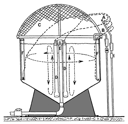
Aquafan’s experimental zero-exchange system (1.82-meter-diameter tank with a sloped bottom and center and wall airlifts) produced a growth rate of 2.16 grams per week, final weight of 19 grams, and survival of 70 percent for a grow-out period of eight weeks at a stocking density of 50 shrimp per square meter (Fig. 1). The system, however, was not capable of producing these growth results at higher stocking densities.

The problem was related to system design. At high densities, shrimp tended to crowd and be funneled down the sloped bottom. Due to water mixing and circulation near the standpipe and airlifts, shrimp were trapped in the area and died.

Design modified

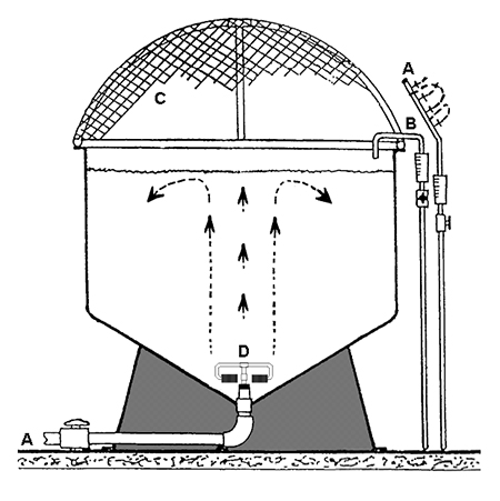
The design was modified by replacing the standpipe and airlifts with T-airstones installed at the bottom center of the tank (Fig. 2). This configuration provided both aeration and water mixing to keep solids in suspension.

Shrimp survival improved to 98 percent, but growth rate was very low (0.7 grams per week). Among other factors, the slow growth was attributed to turbulent water mixing that created inadequate food supply at the tank bottom and caused the shrimp to utilize their energy to maintain balance. Aeration and water mixing also prevented feed pellets from settling and broke the feed into smaller particles that remained in suspension at the water column.

New design

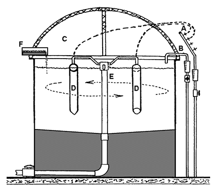
The next experimental zero-exchange design consisted of a circular, flat-bottom tank with airlift pumps attached to the center standpipe (Fig. 3). Aeration rate (1 cfm air per
1,000 liters of water) was configured to produce sufficient water velocity for oxygen supply and water circulation.

Water mixing and feeding

The water mixing was designed to permit feed pellets to settle on the tank bottom, but provide enough current (0.5 to 15 centimeters per second) to agitate them and suspend smaller particles in the water column. Solids agitation prevented build-up of anaerobic conditions on the tank bottom. Water depth could range 60 to 90 cm, as regulated by the height of the center pipe. The feeding unit consisted of an automatic belt feeder that could provide 24-hour continuous feeding or intermittent feeding, if necessary.

Tank cover

The design also incorporated a tank cover. The cover permitted light penetration, but served as a physical barrier for pathogens to increase biosecurity, and provided a more stable environment with high water temperature for conducting experiments.

Solids removal

At high stocking densities, some net removal of particulate solids from the system may be required during shrimp production. To handle this, the system will be equipped with an external filtration system. The materials removed by the solids filter will be quantified and characterized to evaluate its impact on the shrimp and culture system performance. If results indicate that solids removal significantly improves shrimp production, future work will include the development of economical and energy-efficient methods for handling solids.

Shrimp growth and feeding models

The authors evaluated the application of the aquaculture simulation software AquaFarm to the analysis and modeling of an experimental zero-exchange system for the production of Litopenaeus vannamei. The initial focus is on the development of an organismal performance model for shrimp that includes metabolism, feeding, and growth. 

Douglas Ernst’s AquaFarm is a simulation and decision-support software for the design and management planning of finfish and crustacean aquaculture facilities. Scheduled for public release in 2003, it incorporates unit-process and system models that simulate and analyze zero-exchange shrimp production designs.

Growth model

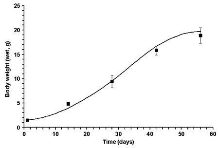
The study used a double-logarithmic shrimp growth model, which is based on the linear relationship between the logarithms of body weight and specific growth rate. To this standard functional form, scalar terms were added for consumption rates and quality of natural and prepared feeds, water temperature, and other water-quality variables that limit growth (e.g., dissolved oxygen and unionized ammonia). For long-term simulations of shrimp production over several months, this model is used over a series of time steps to account for changing culture conditions.

The model is: W_t = [W_o^Ge + (aT + bT²)(G_c G_e S_w S_ft)] ^{(1 per Ge)}, where W_t = final weight (g), W_o = initial weight (g), t = time (days), T = temperature (degrees C), S_w = water quality scalar (range 0-1, function not shown), S_f = feeding rate and feed quality scalar (range 0-1, function not shown), and G_e, G_c, a, and b are function parameters (constants).

Statistical regression analysis of the data was used to calibrate model parameters. Preliminary results indicated the model had the functionality to predict shrimp growth in a zero-exchange system as shown in Fig. 4.

Other feed-related models

A similar approach and set of driving variables are being used to develop a weight-specific feeding rate model. A shrimp metabolism model is also under development. This model, which includes oxygen consumption and metabolite excretion rates, is based on feeding rates, feed composition, and the stoichiometry (bioenergy-based mass balance) of food utilization.

Production system model

The production system model includes the shrimp growth and feeding models, plus additional physical, chemical, and biological elements of the shrimp production system. System-level validation involves shrimp performance, as well as water temperature, pH, dissolved-oxygen levels, total ammonia-nitrogren, algal and detrital solids, and system components.

Feeding rates

Two feeding-rate models are presently being calibrated for shrimp. The models predict feeding rates for appetite satiation as a function of shrimp body weight, temperature, and water quality, and predict the contribution of natural food resources to shrimp feeding.

Analogous in functional form to the double-logarithmic shrimp growth model, the appetite-satiation feeding model is applicable to both prepared and natural feeds. The modeling of natural food resources employs two approaches: a simplified biomass density-productivity model using “critical standing crop” and “carrying capacity” terms, and a more mechanistic approach that quantifies the availability and quality of specific food components (algae, bacterial-detrital aggregate, etc.).

Economic analysis

Economic analysis is another component of the design and modeling work that looks at total system response to alternative feeding regimes and culture system design. It includes the generation of enterprise budgets by simulation and direct cost specifications for alternative feeding regimes, and the evaluation of economic feasibility for alternative production designs. For expanded economic analyses beyond enterprise budgets, a standalone spreadsheet model will be used.

Conclusion

Production models serve as facility design and management tools for understanding the complex nature of aquaculture system. As reflected in the goals of Oceanic Institute’s Aquafan program, they also facilitate technology transfer from researchers to producers.

Modeling analysis and optimization of feed inputs enhance the profitability of pond facilities and reduce resource consumption. Such analyses benefit researchers, extension specialists, producers, and planners in developing pond management regimes that provide maximum benefits for production facilities.

(Editor’s Note: This article was originally published in the June 2002 print edition of the Global Aquaculture Advocate.)